When you have different options with an unknown reward rate, how do you explore the different options to maximize rewards. The name multi-arm bandit comes from considering multiple slot machines with unknown payouts. This problem comes up a lot in the area of web optimization when you are trying to measure if a user takes an action or not. There are many approaches to solving this problem such as ϵ-greedy, softmax, UCB1 and Thompson sampling [1]. The differences between these algorithms is how they decide to explore/exploit arms based on previous results. I’ll go over ϵ-greedy to motivate the basic concept and Thompson sampling for a mathematically precise objective.
The best arm is the arm with the highest historical success rate. At each trial, choose an arm with probability,
| P(best arm) | = 1 - ϵ | ||
| P(other arms) | = ϵ |
The best arm is recomputed after each trial. Each of the other arms are sampled with equal probability. ϵ controls how much time you spend exploring versus exploiting, it is typically chosen to be 0.1. The problem with ϵ-Greedy is that it can get stuck on the bad solution for a while.
A Bernoulli random variable is 1 with a probability p and 0 with a probability q = 1 - p. Usually 1 represents the event occur and 0 represent an event not occurring. This can be expressed with the probability mass function,
For a fair coin, p = 0.5 is the probability of a head appearing (k = 1).
The confidence interval tells you how likely the true p is in a range. We can estimate p by conducting repeated Bernoulli trials.
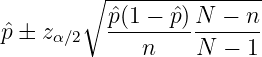
where N is the total population size, n is the sample size,  is the measured
proportion and zα∕2 is the confidence level desired by looking up n in the
t-distribution table.
is the measured
proportion and zα∕2 is the confidence level desired by looking up n in the
t-distribution table.
N is usually large, so finite population correction factor term,
leaving
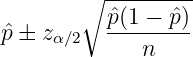
where zα∕2 is read from the normal error integral table as show in Table 1 instead of the t-distribution. For 95% confidence interval, zα∕2 = 1.96, from adding row 1.9 and column 0.06 together.
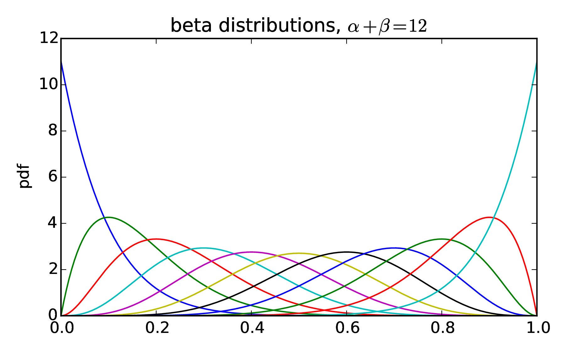
The next building block is the β distribution. The β distribution is the probability distribution of what the true p is based on observations. The probability density function is
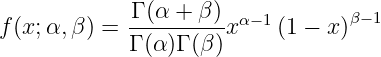
where α,β > 0. Figure 1 shows the distribution for different values of α and β. α - 1 can be thought of as the number of times a trial succeeded and β - 1 the number of times a trial failed. In the beginning, we can assume maximum ignorance. We have no idea if the even always occurs, never occurs or what the chances of occurring would be, so the probability is uniform across all possibilities. If we assume there is chance for the event to occur and a chance for it to not occur, then we can start with α,β = 2. If in the next trial, the even doesn’t occur, we increment β to 3. So, we have 1 event occurring from 3 trials and our β distribution peaking at 1/3. As we get more information from each successful trial, our β distribution shifts.
Thompson sampling is when arms are sampled according the probability that each arm is the best arm [2]. This avoids getting stuck on bad arms and the algorithm will explore arms to get more information about which one is the best.
Each arm can be represented by a β distribution. If we randomly sample each distribution, we can get an estimated value of p. We choose the arm with the highest p. This minimizes the regret since we are choosing the arms with the best chance of being the best. Bad arms will be avoided once enough information is collected and arms with close distributions will be sampled equally until their distributions diverge.
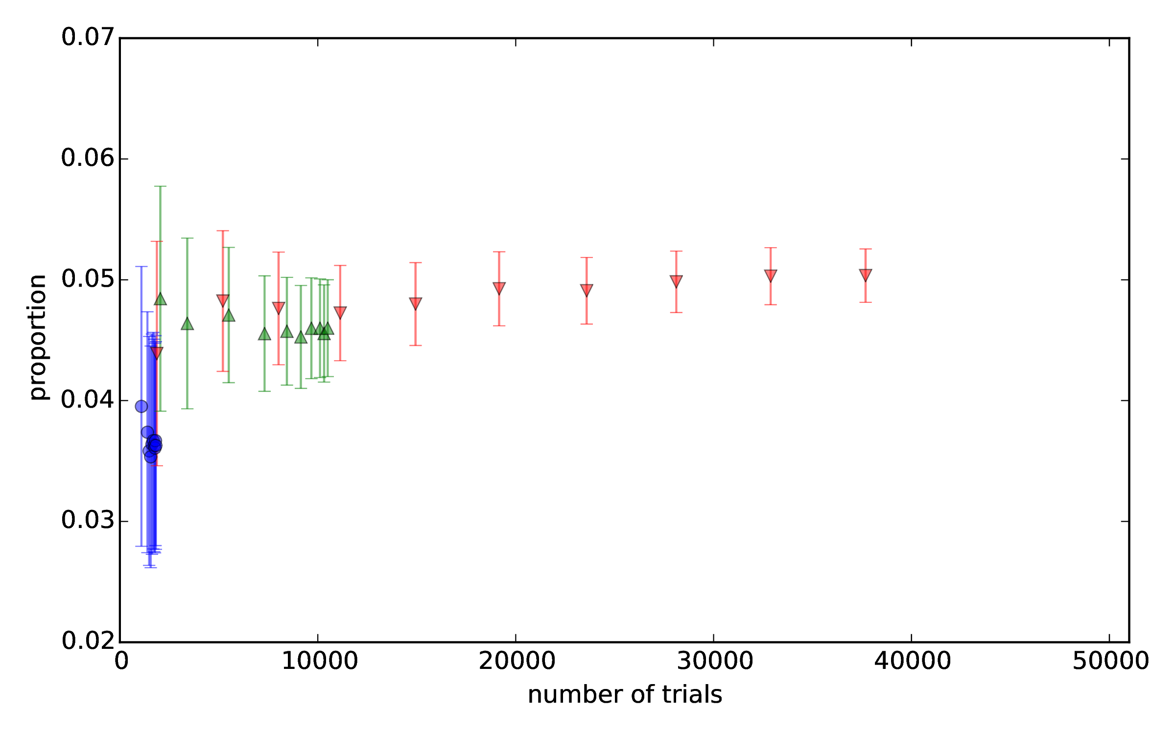
In Python, numpy.random.beta draws samples from a β distribution. The
results of a simulation using Thompson sampling is shown in Figure 2. The
confidence interval decreases with increasing number of trials as  .
.
| t | 0.00 | 0.01 | 0.02 | 0.03 | 0.04 | 0.05 | 0.06 | 0.07 | 0.08 | 0.09 |
| 0.0 | 0.00 | 0.80 | 1.60 | 2.39 | 3.19 | 3.99 | 4.78 | 5.58 | 6.38 | 7.17 |
| 0.1 | 7.97 | 8.76 | 9.55 | 10.34 | 11.13 | 11.92 | 12.71 | 13.50 | 14.28 | 15.07 |
| 0.2 | 15.85 | 16.63 | 17.41 | 18.19 | 18.97 | 19.74 | 20.51 | 21.28 | 22.05 | 22.82 |
| 0.3 | 23.58 | 24.34 | 25.10 | 25.86 | 26.61 | 27.37 | 28.12 | 28.86 | 29.61 | 30.35 |
| 0.4 | 31.08 | 31.82 | 32.55 | 33.28 | 34.01 | 34.73 | 35.45 | 36.16 | 36.88 | 37.59 |
| 0.5 | 38.29 | 38.99 | 39.69 | 40.39 | 41.08 | 41.77 | 42.45 | 43.13 | 43.81 | 44.48 |
| 0.6 | 45.15 | 45.81 | 46.47 | 47.13 | 47.78 | 48.43 | 49.07 | 49.71 | 50.35 | 50.98 |
| 0.7 | 51.61 | 52.23 | 52.85 | 53.46 | 54.07 | 54.67 | 55.27 | 55.87 | 56.46 | 57.05 |
| 0.8 | 57.63 | 58.21 | 58.78 | 59.35 | 59.91 | 60.47 | 61.02 | 61.57 | 62.11 | 62.65 |
| 0.9 | 63.19 | 63.72 | 64.24 | 64.76 | 65.28 | 65.79 | 66.29 | 66.80 | 67.29 | 67.78 |
| 1.0 | 68.27 | 68.75 | 69.23 | 69.70 | 70.17 | 70.63 | 71.09 | 71.54 | 71.99 | 72.43 |
| 1.1 | 72.87 | 73.30 | 73.73 | 74.15 | 74.57 | 74.99 | 75.40 | 75.80 | 76.20 | 76.60 |
| 1.2 | 76.99 | 77.37 | 77.75 | 78.13 | 78.50 | 78.87 | 79.23 | 79.59 | 79.95 | 80.29 |
| 1.3 | 80.64 | 80.98 | 81.32 | 81.65 | 81.98 | 82.30 | 82.62 | 82.93 | 83.24 | 83.55 |
| 1.4 | 83.85 | 84.15 | 84.44 | 84.73 | 85.01 | 85.29 | 85.57 | 85.84 | 86.11 | 86.38 |
| 1.5 | 86.64 | 86.90 | 87.15 | 87.40 | 87.64 | 87.89 | 88.12 | 88.36 | 88.59 | 88.82 |
| 1.6 | 89.04 | 89.26 | 89.48 | 89.69 | 89.90 | 90.11 | 90.31 | 90.51 | 90.70 | 90.90 |
| 1.7 | 91.09 | 91.27 | 91.46 | 91.64 | 91.81 | 91.99 | 92.16 | 92.33 | 92.49 | 92.65 |
| 1.8 | 92.81 | 92.97 | 93.12 | 93.28 | 93.42 | 93.57 | 93.71 | 93.85 | 93.99 | 94.12 |
| 1.9 | 94.26 | 94.39 | 94.51 | 94.64 | 94.76 | 94.88 | 95.00 | 95.12 | 95.23 | 95.34 |
| 2.0 | 95.45 | 95.56 | 95.66 | 95.76 | 95.86 | 95.96 | 96.06 | 96.15 | 96.25 | 96.34 |
| 2.1 | 96.43 | 96.51 | 96.60 | 96.68 | 96.76 | 96.84 | 96.92 | 97.00 | 97.07 | 97.15 |
| 2.2 | 97.22 | 97.29 | 97.36 | 97.43 | 97.49 | 97.56 | 97.62 | 97.68 | 97.74 | 97.80 |
| 2.3 | 97.86 | 97.91 | 97.97 | 98.02 | 98.07 | 98.12 | 98.17 | 98.22 | 98.27 | 98.32 |
| 2.4 | 98.36 | 98.40 | 98.45 | 98.49 | 98.53 | 98.57 | 98.61 | 98.65 | 98.69 | 98.72 |
| 2.5 | 98.76 | 98.79 | 98.83 | 98.86 | 98.89 | 98.92 | 98.95 | 98.98 | 99.01 | 99.04 |
| 2.6 | 99.07 | 99.09 | 99.12 | 99.15 | 99.17 | 99.20 | 99.22 | 99.24 | 99.26 | 99.29 |
| 2.7 | 99.31 | 99.33 | 99.35 | 99.37 | 99.39 | 99.40 | 99.42 | 99.44 | 99.46 | 99.47 |
| 2.8 | 99.49 | 99.50 | 99.52 | 99.53 | 99.55 | 99.56 | 99.58 | 99.59 | 99.60 | 99.61 |
| 2.9 | 99.63 | 99.64 | 99.65 | 99.66 | 99.67 | 99.68 | 99.69 | 99.70 | 99.71 | 99.72 |